Scalability Profiling
Overview
Teaching: 0 min
Exercises: 0 minQuestions
How scalable is a particular piece of code?
How can I generate evidence for a code’s scalability?
What does good and bad scalability look like?
Objectives
Explain how Amdahl’s Law can help us understand the scalability of code.
Use Amdahl’s Law to predict the theoretical maximum speedup on some example code when using multiple processors.
Understand strong and weak scaling graphs for some example code.
Describe the graphing characteristics of good and bad scalability.
Let’s look at how we can determine the scalability characteristics for some example code.
Calculating π as an Example
In the following example we have a simple piece of code that calculates π. When run on our local system we get the following results:
| Cores (n) | Run Time (s) | Result | Error | Speedup |
|---|---|---|---|---|
| 1 | 3.99667 | 3.141592655 | 0.00000003182 | - |
| 2 | 2.064242 | 3.141592655 | 0.00000003182 | 1.94 |
| 4 | 1.075068 | 3.141592655 | 0.00000003182 | 3.72 |
| 8 | 0.687097 | 3.141592655 | 0.00000003182 | 5.82 |
| 16 | 0.349366 | 3.141592655 | 0.00000003182 | 11.44 |
How is our program parallelised?
Our π program uses the popular Message Passing Interface (MPI) standard to enable communication between each of the parallel portions of code, running on separate CPU cores. It’s been around since the mid-1990’s and is widely available on many operating systems. MPI also is designed to make use of multiple cores on a variety of platforms, from a multi-core laptop to large-scale HPC resources such as those available on DiRAC. There are many available tutorials on MPI.
By using MPI, we can reduce the run time of our code by using more cores, without affecting the results. The speedup shown in the table above was calculated using:
Speedup = T1 / Tn
What Type of Scaling?
Looking at the table above, is this an example of determining strong or weak scaling?
Solution
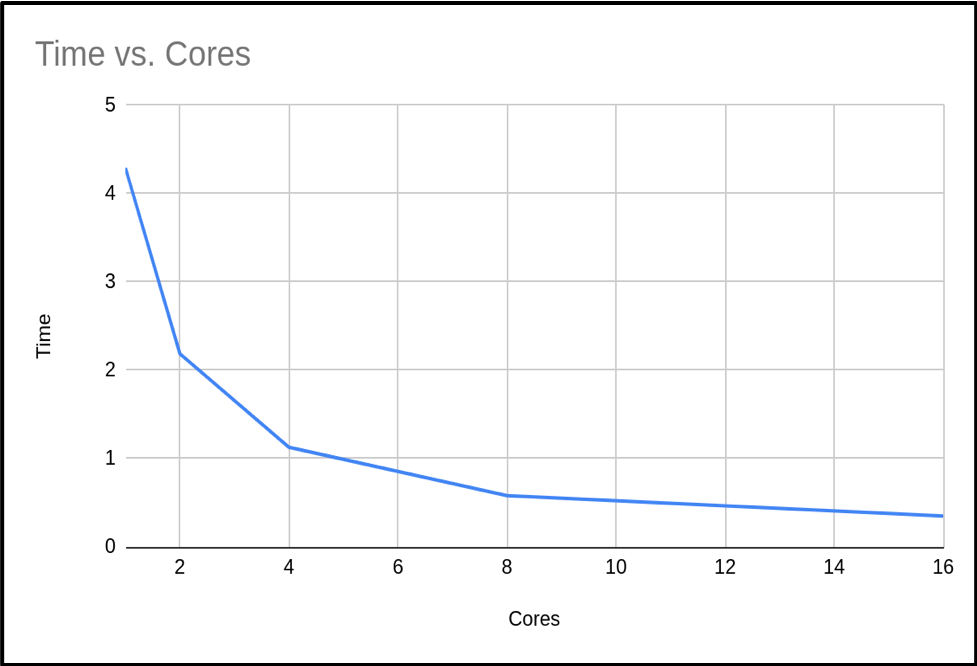
This is an example of strong scaling, as we are keeping the data sample the same but increasing the number of cores used.
When we plot the run time against the number of cores, we see the following graph:
Determining Serial and Parallel Proportions of Code
We can use Amdahl’s Law to give us a theoretical indication of the speedup possible by using more cores when running our code. In order to do this, we need an idea of what proportions of our code are in executed in serial and parallel. It is oftentimes difficult to estimate the proportion of serial code, but we can estimate this by using Amdahl’s Law.
Assuming:
Time to Complete (T) = Time taken for Serial Portion (S) + Time taken for Parallel Portion (P)
T = S + P
To help us solve this, we can write the parallel portion P as T - S. This gives us:
T = S + ( T - S )
We will assume, for simplicity, that the time it takes to run the serial portion is constant, and that only the parallel portion of the code is affected when we increase the number of cores in use. Therefore, using 2 cores we can rewrite Amdahl’s law as:
T2 = S + ( T1 - S ) / 2
And in general, for n cores:
Tn = S + ( T1 - S ) / n
We can now rearrange this to solve for S, the time taken for the serial portion of our code:
S = ( nTn - T1 ) / (n - 1)
Using the above formula on our example code we get the following results:
| Cores (n) | Tn | Sn | Pn = (Tn - Sn) | Serial % | Parallel % |
|---|---|---|---|---|---|
| 1 | 3.99667 | - | - | - | - |
| 2 | 2.064242 | 0.131814 | 1.932428 | 6.39 | 93.61 |
| 4 | 1.075068 | 0.101200 | 0.973867 | 9.41 | 90.59 |
| 8 | 0.687097 | 0.214300 | 0.472796 | 31.20 | 68.81 |
| 16 | 0.349366 | 0.106212 | 0.243153 | 30.40 | 69.60 |
| Average | 19.35 | 80.65 |
We now have an estimated percentage for our serial and parallel portion of our code. Ss you can see, as the number of cores we use increases, the percentage of the run time spent in the serial portion of the code increases.
Differences in Serial Timings
You may be wondering why the serial run time seems to vary depending on the run. There are several factors that are impacting our code. Firstly these were run on a working system with other users, so runtime will be affected depending on the load of the system. Throughout DiRAC, it is normal when you run your production code to have exclusive access to the servers, so this will be less of an issue. But if, for example, your code accesses bulk storage then there may be an impact since these are shared resources. As we are using the MPI library in our code, it would be expected that the serial portion will actually increase slightly with the number of cores due to additional MPI overheads. This will have a noticeable impact if you try scaling your code into the thousands of cores.
What’s the Maximum Speedup?
We can use these figures to give us the theoretical maximum possible speed up we could achieve:
Speedup = T1/Tn
And
Tn = S + (T1 - S) / n
For simplicity and when using percentages we normally set T1 to 1. Therefore we will get a speedup relative to 1.
Therefore:
Speedup = 1 / Tn
Tn = S + ( 1 - S ) / n
As we increase the number of cores to infinity, then Tn approaches S.
Tn = S
Max Speedup = 1 / S
And in our case:
Max Speedup = 1 / 19% => 5
Number of Cores vs Expected Speedup
Using Amdahl’s Law and the percentages of serial and parallel proportions of our example code. Fill In or create a table estimating the expected total speedup and change in speedup when doubling the number of cores, in a table like the following (with the number of cores doubling each time until a total of 4096):
Cores (n) Tn Speedup Change in Speedup 1 3.99667 2 4 … 4096 Solution
Hopefully from your results you will find that we can get close to the maximum speedup of 25, but it requires ever more resources.
Speedup Change?
When does the change in speedup drop below 1%?
Solution
From our own trial runs this happens at 4096 core, but it is expected that we would never run this code at these core counts as it would be a waste of resources.
How Many Cores Should we Use?
From the data you have just calculated, what do you think the maximum number of cores we should use with our code to balance reduced execution time versus efficient usage of compute resources.?
Solution
Within DiRAC we do not impose such a limit, this would be a decision made by the researchers. Every project has an allocation and it is up to you to decide what is efficient use of your allocation. In this case I personally would not waste my allocation on any runs over 128 cores.
Calculating a Weak Scaling Profile
Not all codes are suited to strong scaling. As seen in the previous example, even codes with as much as 96% parallelizable code will hit limits. Can we do something to enable moderately parallelizable codes to access the power of HPC systems? The answer is yes, and is known as weak scaling.
The problem with strong scaling is as we increase the number of cores, then the relative size of the parallel portion of our task reduces until it is negligible, and then we can not go any further. The solution is to increase the problem size as you increase the core count – this is Gustafson’s law. This method tries to keep the proportion of serial time and parallel time the same. We will not get the benefit of reduced time for our calculation, but we will have the benefit of processing more data. Below is a re-run of our π code. But this time, as we increase the cores we also increase the samples used to calculate π.
| Cores (n) | Run Time | Result | Error | % Improved Error |
|---|---|---|---|---|
| 1 | 4.149807 | 3.141592655 | 0.00000003182 | |
| 2 | 4.362416 | 3.141592654 | 0.00000001591 | 50.00% |
| 4 | 5.205988 | 3.141592654 | 0.00000000795 | 75.02% |
| 8 | 4.356564 | 3.141592654 | 0.00000000397 | 87.52% |
| 16 | 4.643724 | 3.141592654 | 0.00000000198 | 93.78% |
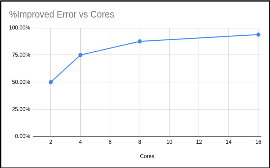
As you can see, the run times are similar. Just slightly increasing. However, the accuracy of the calculated value of π has increased. In fact our percentage improvement is nearly in step with the number of cores.
When presenting your weak scaling it is common to show how well it scales, this is shown below:
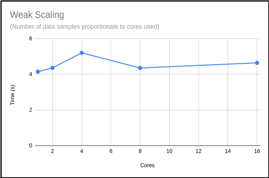
We can also plot the scaling factor. This is the percentage increase in run time compared to base run time for a normal run. In this case we are just using T1:
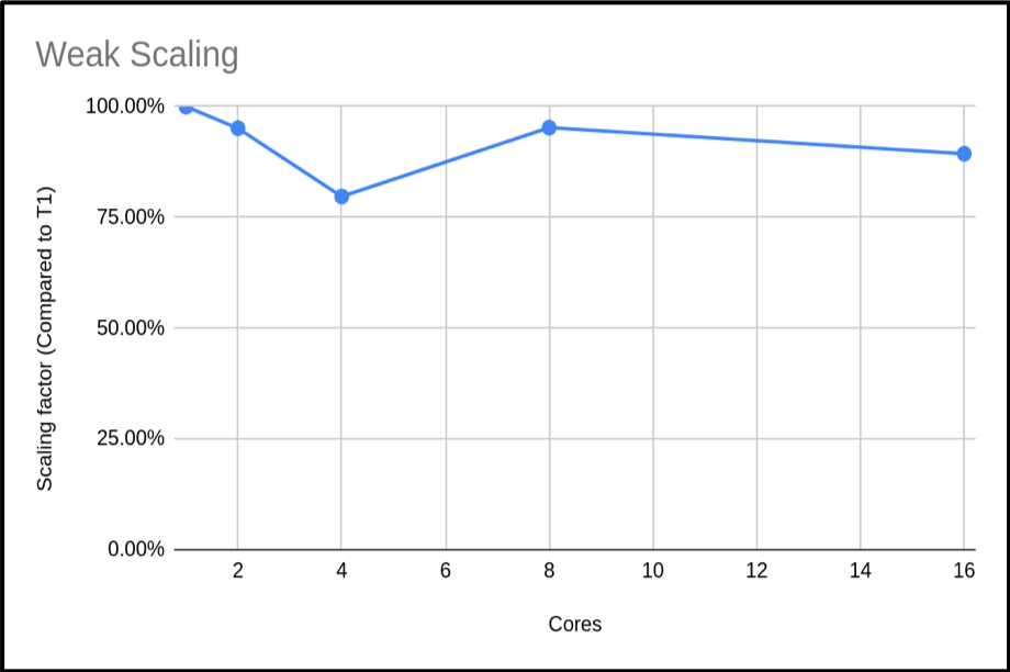
The above plot shows that the code is highly scalable. We do have an anomaly with our 4 core run, however. It would be good to rerun this to get a more representative sample, but this result is a common occurrence when using shared systems. In this example we only did a single run for each core count. When compiling your data for presentation or submitting applications, it would be better to do many runs and exclude outlying data samples or provide an uncertainty estimate.
Maximum Cores to Use?
It would be hard to estimate the max cores we could use from this plot. Can you suggest an approach to get a clearer picture of this code’s weak scaling profile?
Solution
The obvious answer is to do more runs with higher core counts, and also try to resolve the n = 4 sample. This should give you a clearer picture of the weak scaling profile.
Obtaining Resources to Profile your Code
It may be difficult to profile your code if you do not have the resources at hand, but DiRAC can help. If you are in a position of wanting to use DiRACs facilities but do not have the resources to profile your code, then you can apply for a Seedcorn project. This is a short project with up to 100,000 core hours for you to profile and possibly improve your code before applying for a large allocation of time.
Profiling Pi Yourself
If you would like to reproduce these sample runs on your system, the code is available on the DiRAC GitHub page.
Key Points
We can use Amdahl’s Law to understand the expected speedup of a parallelised program against multiple cores.
It’s often difficult to estimate the proportion of serial code in our programs, but a reformulation of Amdahl’s Law can give us this based on multiple runs against a different number of cores.
Run timings for serial code can vary due to a number of factors such as overall system load and accessing shared resources such as bulk storage.
The Message Passing Interface (MPI) standard is a common way to parallelise code and is available on many platforms and HPC systems, including DiRAC.
When calculating a strong scaling profile, the additional benefit of adding cores decreases as the number of cores increases.
The limitation of strong scaling is the fixed problem size, and we can increase the problem size with the core count to obtain a weak scaling profile.